Setup:

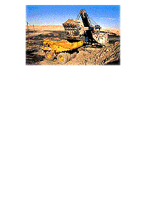
Using a programmable digital camera, we took pictures at a distance of 1.67 meters from photographed object (in this case a comic book cover).   We then implemented the autofocusing program in Labview, a graphical programming environment.

Camera used: Tiffen Lens 49mm Hot Mirror USA
Light source: Lowel Omni  500W, 8.4Amp, 12V, 50/60 Hz

     Implementation:

The decision logic was implemented as follows:

    User specifies algorithm to use (choice of Squared Gradient, Absolute Variation, or Laplacian)
    User specifies distance to begin trial auto-focusing (example: begin at 1.2m from camera)
    User specifies initial increment to begin auto-focusing process
    User specifies tolerable difference threshold in focus measure units
    The chosen algorithm decides at each increment during the auto-focusing process, if the new image is focused within the specified difference threshold
    If the image is not yet focused satisfactorily, the program calls for the object distance to be changed by first the user-specified initial increment, then each  subsequent increment/decrement  pair will change by half of the previous pairs' increment/decrement.
 

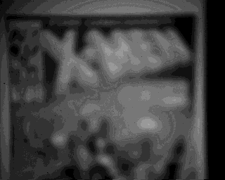
Picture is taken at 1.67 meters from the camera (object distance), with aforementioned camera and light source.

User specs:  Squared Gradient algorithm for focus measure, 1.2 m beginning comparison distance, 0.4 m initial increment, 1x10^6  difference threshold*

*note: for Squared Gradient algorithm, threshold tolerance is especially large, and 1x10^6  is typical for difference threshold

To view the progression of auto-focus images, refer to the picture below, which  scrolls through a series of 8 pictures, beginning at 1.2 m object distance, with initial increment of 0.4 m.  After comparison of images at 1.2 m and 1.6 m, the algorithm decides the image is not yet sufficiently focused, i.e. does not satisfy user-specified threshold.  A comparison of images is then done for 2.0 m and 1.6 m.  This continues as the increment is halved to 0.2 m, and a comparison is made between images taken at 1.6 m and 1.8m.   We finally see that the difference threshold criteria is fulfilled at 1.725 m.

*The images are presented for 1.5 seconds each--the last image is displayed for 5 seconds to distinguish it from the remainder of the cycle.
 
 

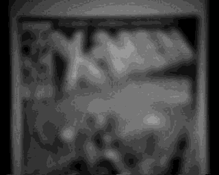
Now, the same demonstration for the Laplacian algorithm:
 
 

Finally, the Absolute Variation algorithm implementation:
 
 

 back