
![]() What is auto-focusing?
What is auto-focusing?
The sharpness of an image is the determining factor in human visual perception of focus. Upon examining the frequency components of an unfocused image, you will find that there are relatively few high frequency components. As the image comes into focus, high frequency components increase.
In analog cameras, auto-focusing is done manually, with a sensor which actually measures distance (object distance) to the photographed object. In digital cameras, as mentioned in the Motivation section, signal processing (computational power) may be leveraged to enable auto-focusing.
The lens of a camera is essentially a low pass filter, which focuses by shifting the cutoff frequency of the filter to the higher frequency side. In digital cameras, the software controls the lens position, maximizing higher frequency components. The term focus measure refers to the metric by which we measure the amount of high frequency components--maximum focus measure occurs when the image is most closely focused.
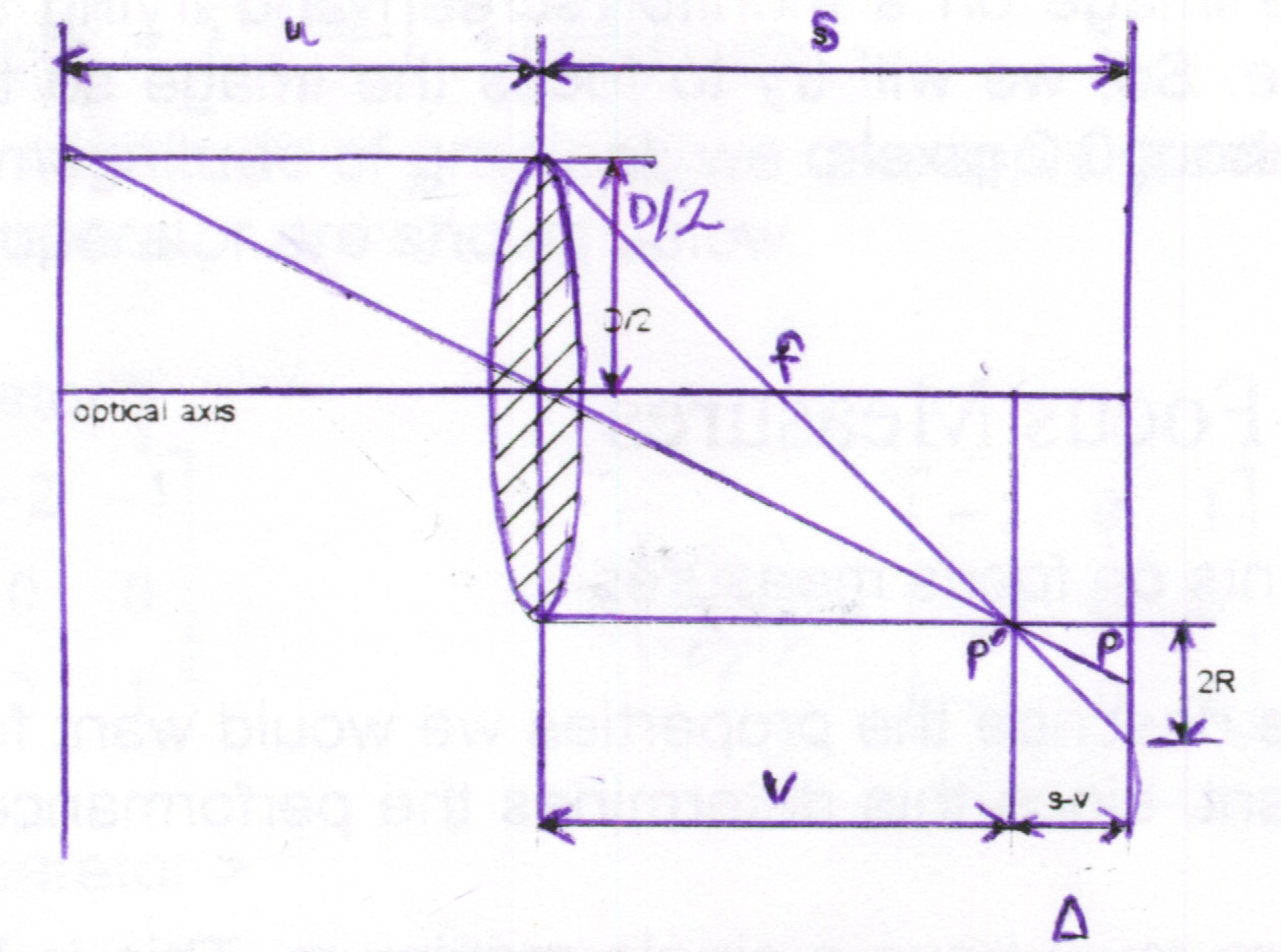
![]() A Simple focus model for reference purposes:
A Simple focus model for reference purposes:
The picture below models a simple optic system.
R = | (s-v)*D / (2v) | = | delta*D / (2v) |
When the blur radius is less than 0.4 pixels, the blurred and focused images are difficult to distinguish.
![]() What are focus measures?
What are focus measures?
Focus measures are the algorithms by which we determine
when an image is "focused."
Several examples of such algorithms will be presented
in this section. In the meantime, let us discuss critical properties
of focus measures in general. It is important that a focus measure
be unimodal, i.e. that it have one and only one single maximum value.
Multiple maxima can lead to large focus error, as the focus measure algorithms
essentially judge a image to be in focus at the maximum value of the function.
Local maxima would skew results. Large variation of value due to
changes in distance from focused to current image plane positively affects
accuracy of the focus measure. Large usable range is a useful quality
in that it allows the focus measure to work even in extremely defocused
situations. Finally, a good focus measure ideally has minimal computation
complexity, to minimize computational load. Well-chosen focus measures
are also insensitive to mean brightness and noise.
where g(i, j) is the gray-value at pixel (i,j) in a given square image of size N x N.
Absolute Gradient works for images in which the objects
to bring into focus are small compared to the size of the point spread
function. It is one of the simplest focus measure algorithms, and
focuses pictures with many edges well.
where g(i, j) is the gray-value at pixel (i,j) in a given square image of size N x N.
Through squaring, we weigh the larger gradients more heavily
than the smaller ones. This method is one of the most flexible, and
deals well with images with many edges, high or low mean brightness, and
dark or light background. This algorithm also offers the advantages
of robustness to noise and good range.
where g(i, j) is the gray-value at pixel (i,j) in a given square image of size N x N.
While the Laplacian method has excellent accuracy, it
is highly sensitive to noise. In the frequency domain, the Laplacian
may be modeled as a second order difference filter, as such it more strongly
kills off lower spatial frequencies than first order difference filters
such as that implemented by the gradient functions.
where g(i, j) is the gray-value at pixel (i,j) in a given square image of size N x N.
Absolute variation is a simplified version of standard
deviation, which requires greater computational load. In general,
the standard deviation algorithm is frequently used due to its flexibility
(it, like the squared gradient method, is relatively immune to mean brightness,
background brightness, high edge count).