JPEG Compression in the Intensity Domain
S-CIELAB
The most significant statistic is the number of points above noticeable
threshhold. In this case, we set the threshhold to 10 CIELAB levels. In
brief, the data below indicates that, by the S-CIELAB metric, the Y-JPEG
method is slightly worse. The total number of pixels for which the Y-JPEG
reproduces better than the regular JPEG is slightly higher, but on the
whole, they are about the same. We can infer from the statistics that the
standard deviation is higher for the Y-JPEG compression.
| |
Mean S-CIELAB error |
Number of points above 10 error levels |
Number of points error level is higher than
other method |
| JPEG |
5.0610 |
7737 |
33541 |
| Y-JPEG |
5.5231 |
9687 |
30459 |
It is important to realize the limitation of the S-CIELAB metric as used
in this experiment. The images below depict the the points in the image
for which the CIELAB errors exceeded 10. Notice the high frequency
nature of the errors in both cases: they lie in areas of high detail and
edges. The errors in the high detail areas are of little consequence; the
edges are slightly more important. But in both cases, because the color
sensitivity of the human eye is much lower than the black-and-white
sensitivity, these differences are not very important. The purpose of
this part of the experiment is to see if there are significant color
distortions. Few are expected, and few are observed. The problem arises
in areas of constant low intensity, due to quantization error.
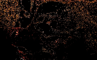
Error of JPEG above 10 CIELAB level |
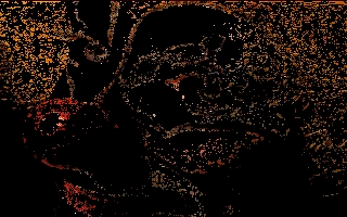
Error of Y-JPEG above 10 CIELAB levels |
Mean Levels
The intention of this Y-JPEG compression scheme was to conserve mean
levels of intensity. The best way to evaluate this is to evaluate each
basic block of the JPEG compression: the 8x8 block. We find that, on
average, the Y-JPEG scheme conserves the mean better. However, if you
take the absolute value of the intensity errors, the Y-JPEG scheme
faares no better than the JPEG in conserving mean. Most
importantly. on average, the error corresponds to less than a graylevel value, and so the advantage of the
Y-JPEG scheme is not perceptually noticeable.
| |
Mean error |
Mean absolute error |
Number of points above error level is higher than
other method |
| JPEG |
-0.0037 |
0.0042 |
394 |
| Y-JPEG |
-0.0003 |
0.0040 |
542 |
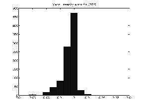
Mean intensity error of JPEG |
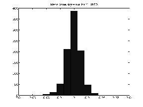
Mean intensity error of Y-JPEG |
We should note that the sinusoidal test images originally shown were about
the minimum mean intensity level for which Y-JPEG was noticeably better.
The mean graylevel of the low contrast image was .9. The mean
graylevel of this image, by comparison, was 0.16. Even this fairly bright
image of parrots had a mean graylevel of
0.23.
Noticeable Artifacts
The CIELAB metric reports color differences that are too high frequency to
notice. On the opposite extreme, the DC intensity discrepancies are also
minimal. However, the quantizing the DCT coefficients in the intensity
domain causes severe false contours in dark regions. Because the
coefficients represent spatial frequencies, there is no way to convert
back to framebuffer values before quantizing short of distorting the
actual cosine waves used by the DCT.
The edge detectors in MATLAB do not notice the false contours. Although
the mean intensity level in the low intensity regions is more likely to be
inaccurate due to the quantization, this is not the main source of error.
Ultimately, none of the tests I derived satisfactorily quanitified the
error, but certainly, these quantization artifacts are the one serious
problem with the Y-JPEG scheme.

B&W of original image |

B&W of JPEG image |
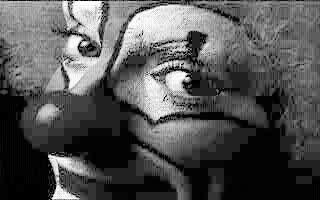
B&W of Y-JPEGimage |
If you have questions or comments, please e-mail Alan Tseng / alant@stanford.edu.