Psychology 221    (This Web page was written by Ali Abbas  as part of a group project)  Supervised  by Prof. Brian Wandell Determining the Sensor responsivities of the Sony Digital Camera ( DSC-F1)      

---

Sensor Responsivity of the SONY DSC-F1 Digital Still Camera

---

 

It is divided into :

2) Data Analysis

3) Camera Prediction

4) Picture Samples

5) Related links
 
 
 

1) Data Gathering:
 

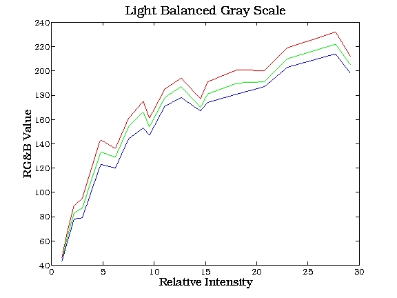
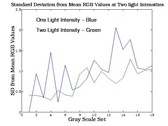
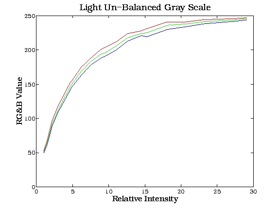
 a) (1 - 20) Gray Scale was used to determine the gamma function .
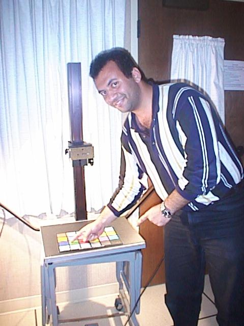
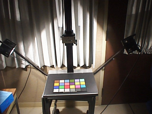
The setup for this experiment is shown below:
As shown, it is an apparatus with camera fixing capability to a predetermined distance from the target and has the ability to supply two different light intensities.
The T

And  so these values were used for determining the Gamma Correction Factor.n
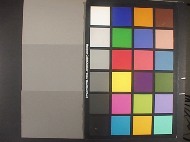
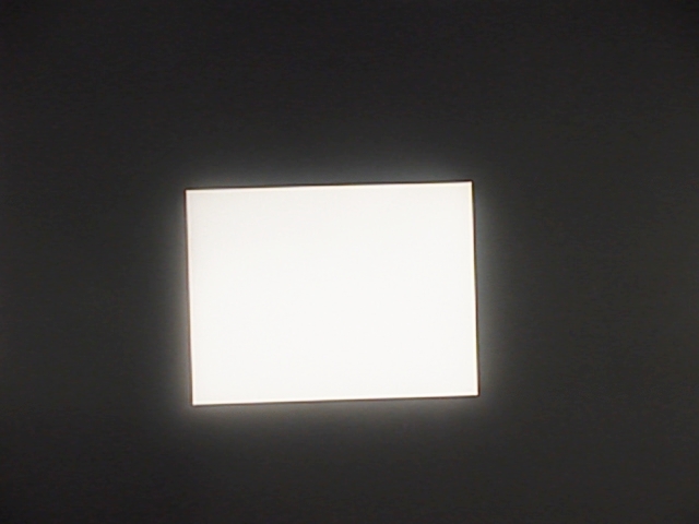
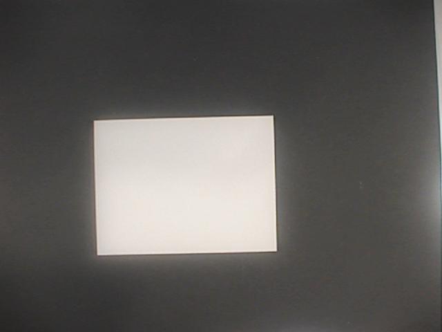
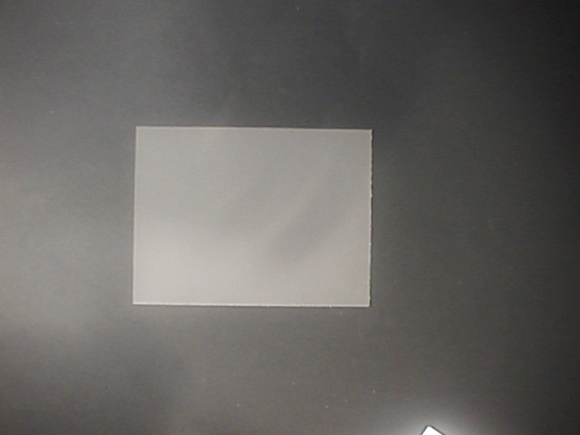
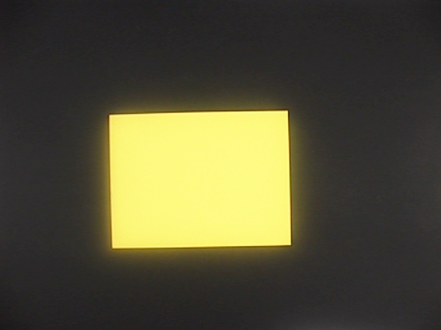
Examples of Gray scale images with the higher light intensity are shown below:
 

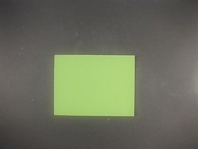
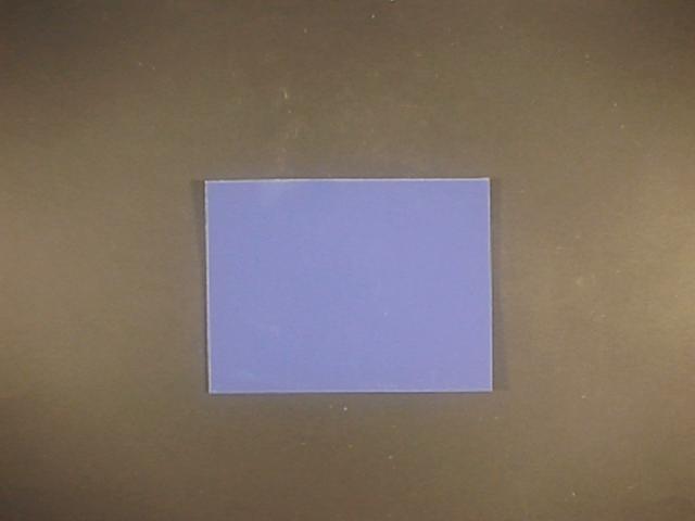
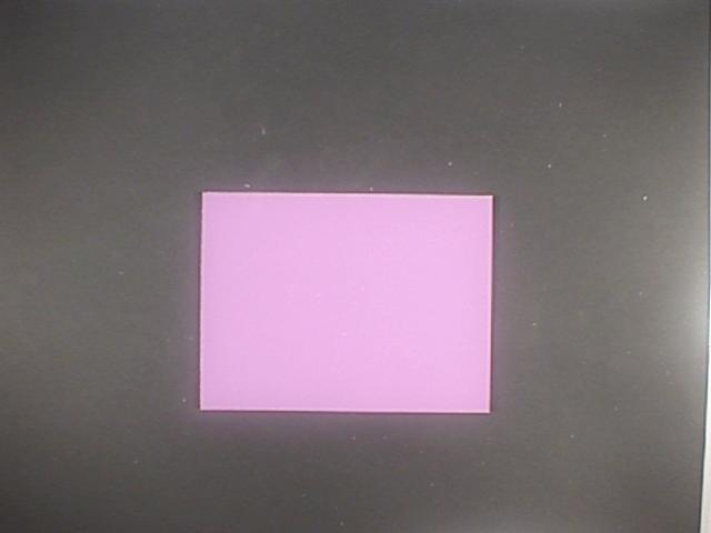
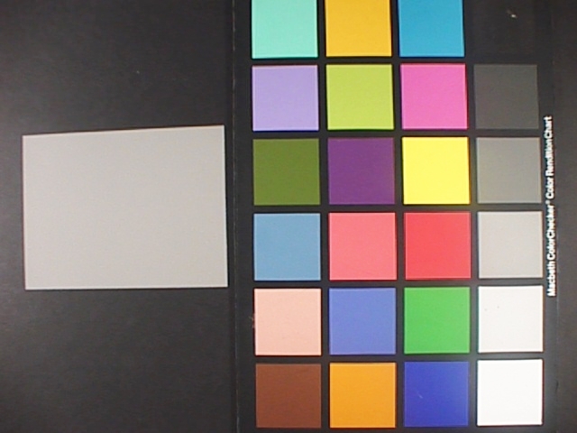
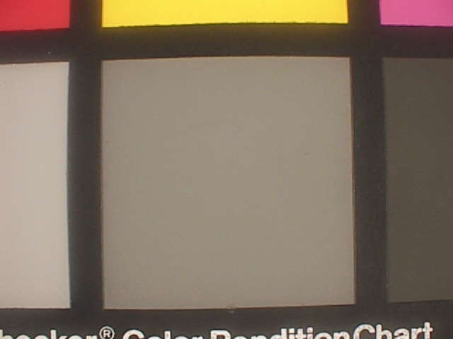
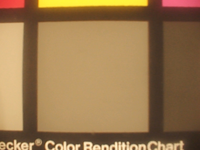
b) The same type of measurements was made for 100 color images and each of these was corrected for the gamma factor.
Samples of these colors are shown below:

c) The Power spectral density for each of these colors was also measures using a Spectral radiometer giving power spectral density  up to 101 wavelengths. The Spectral Radiometer measurement was made using the exact same set up for the DSC-F1 and with the same light intensity and background. 
 
 
 

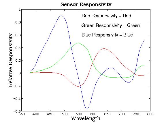
a) The Corrected ( Linearized) RGB values were then used in conjunction with the Spectral Density measurements to obtain a responsivity matrix as explained below:

   [ Linear RGB ] = [ Responsivity ( wavelength) ] [ Spectral Power Density ]

This Responsivity matrix obtained by solving the equation above is a 3*101 matrix that is plotted below:
 

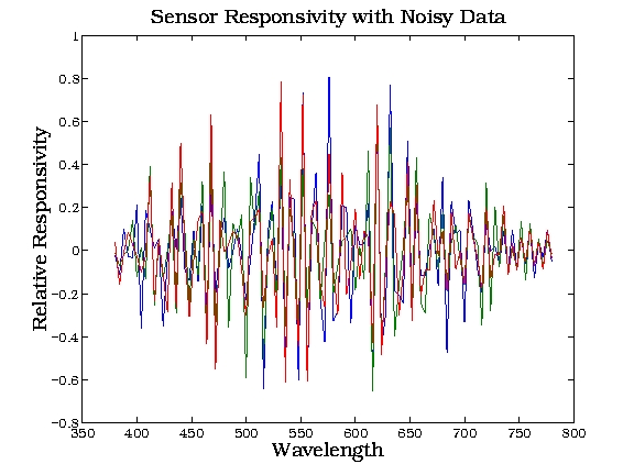
The matrix is very noisy as shown above, but this can be explained due to the sensitivity of the measurements and the actual data matrix can be reduced to lower order matrix through processing of the resulted data.( Acknowledgment here given to Professor Brian Wandell for suggesting this method to us. )
 

b) Processing the data:
We will try to filter out the noisy data using the following procedure:
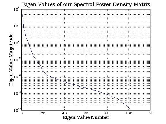
1) Resolve the data matrix into three components ( Two orthogonal matrices U,V and one diagonal matrix S)

    [ D ] = [ U ] [S] [V]

An interesting feature about the diagonal matrix [S] is that the larger numbers are in the top left ends of the diagonal and decrease towards the bottom right ends of the diagonal . This result is plotted below:

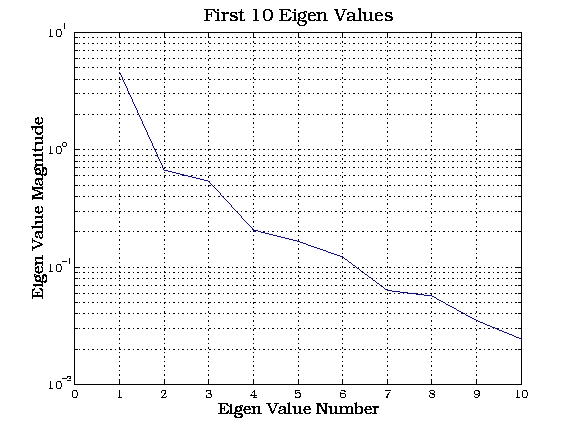
A cut-off value is chosen for the first 5 elements in the diagonal matrix [S] and so the remaining values will be assumed zero.
This effectively reduces the dimensions of the orthogonal [U] matrix into 5 columns.
Solving the matrix equation with the new value of the data matrix now results in a smoother response as shown below
 

An initial attempt gave Problems between predicted values and measured values as shown below:
  

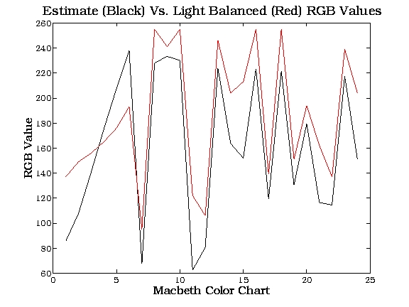
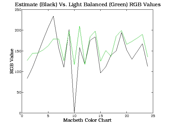
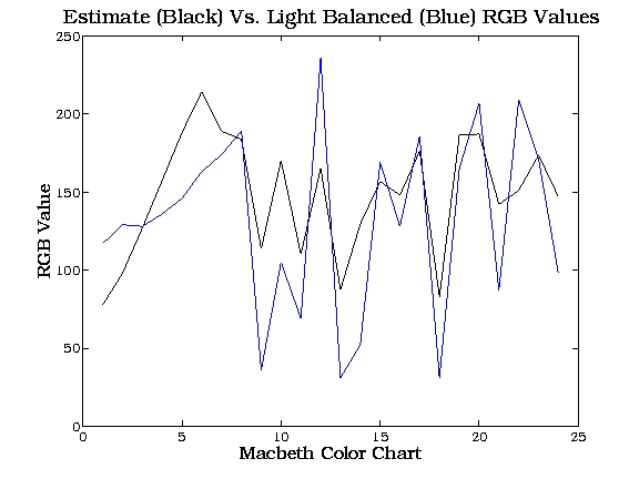
This was mainly due to light balancing made by the camera as every color was measured separately at a distance of 3 inches from the Macbeth checker.
 

The full Macbeth checker was then pictured, to prevent color balancing effect,  and the values of the colors were all obtained from this image. The match between measured and predicted was thus much closer as shown below:

  
 
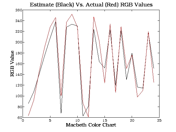
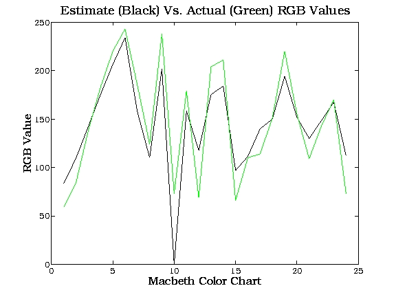
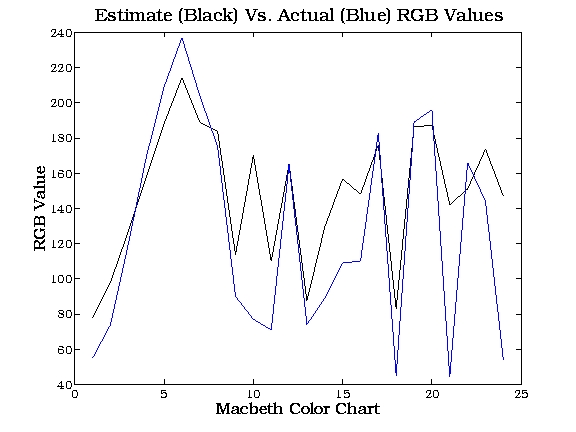
 The average and standard deviation of the error ( Measured - Estimated ) is plotted below for both actual and light-balanced measurements are tabulated below:
 
 

 This was performed to prevent color balancing of the camera due to a single Gray Scale.