At this point, the SPD data from the radiometer had been adjusted for the tungsten light, and the RGB output from the camera had been "unbalanced" and had the gamma correction nonlinearity removed. We knew that the formula for calculating the RGB output from the SPD's was as follows.
RGB = SPD2RGB * SPD
SPD2RGB is the matrix which describes the color matching functions that we are looking for. The RGB values and SPD values were also stored in matrix form. As there were 84 wavelengths at which data was sampled, and 113 color swatches, the matrix multiplication looked something like the following.
RGB [3 x 113] = SPD2RGB [3 x 84] * SPD [84 x 113]
The most direct method of finding SPD2RGB is
SPD2RGB = SPD * inv(RGB)
This plot was very noisy, so it was necessary to do some extra processing to clean it up. We used two methods of noise reduction. First, we manipulated the equations in the following way, which caused Matlab's numeric matrix division function to find a best fit result using a least-squares approach. Second, we reduced the data and recreated the curves using a set of basis functions, using Matlab code provided by Dr. Wandell.
Our manipulations were as follows:
SPD2RGB = RGB * inv(SPD) = RGB / SPD (matlab notation)
RGB * inv(SPD) = inv(SPD * inv(RGB))
SPD * inv(RGB) = SPD / RGB (matlab notation)
=> SPD2RGB = inv(SPD / RGB) (This is the actual calculation done by our Matlab code.)
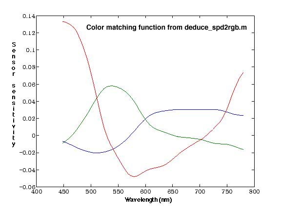
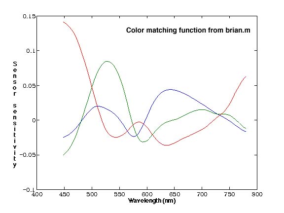
The two methods produced the following sensor estimations. They are very
similar though. Our functions are based on our entire data set, while the
ones calculated by Professor Wandell's methods are based on fewer
representative values.
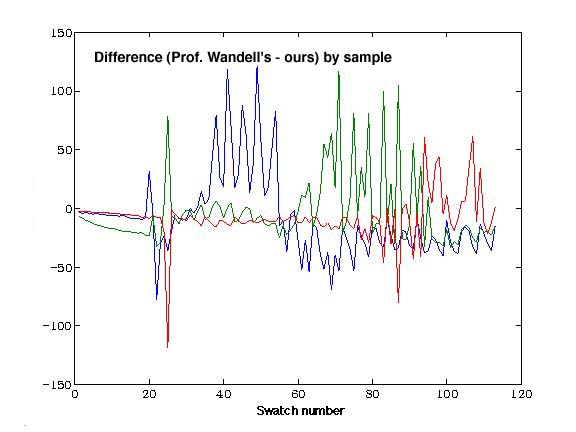
The difference between the two functions is shown here. It is interesting
to note the frequency differences apparent in the two.
One conjecture as to why this occurs looked at the colors of the original
swatches. They are ordered to some extent by hue, and then within this
ordering, their intensity oscillates.